---

Introduction

In this article, we will be using Rain in Australia Dataset from Kaggle. The problem is to predict whether it will rain tomorrow or not given the weather conditions of today. We will be using Decision Tree Classifier in this article.

Index

1. Problem Statement

2. Dataset Description

3. Importing Libraries

4. Configuration

5. Import Dataset

6. Train, Validation, Test Split

7. Identify Inputs & Target Columns

8. Identify Numerical & Categorical Columns

9. Impute Missing Values

10. Scaling Numerical Columns

11. Encoding Categorical Columns

12. Training & Visualizing Decision Trees

13. Feature Importance

14. Hyperparameter Tuning - To Reduce Overfitting

1. Problem Statement

Predict next-day rain by training classification models on the target variable.

2. Dataset Description

The dataset is taken from Kaggle. This dataset contains about 10 years of daily weather observations from many locations across Australia.

Column Description :

• Date : The date of observation

• Location : The common name of the location of the weather station

• MinTemp : The minimum temperature in degrees celsius

• MaxTemp : The maximum temperature in degrees celsius

• Rainfall : The amount of rainfall recorded for the day in mm

• Evaporation : The so-called Class A pan evaporation (mm) in the 24 hours to 9am

• Sunshine : The number of hours of bright sunshine in the day.

• WindGustDir : The direction of the strongest wind gust in the 24 hours to midnight

• WindGustSpeed : The speed (km/h) of the strongest wind gust in the 24 hours to midnight

• WindDir9am : Direction of the wind at 9am

• WindDir3pm : Direction of the wind at 3pm

• WindSpeed9am : Wind speed (km/hr) averaged over 10 minutes prior to 9am

• WindSpeed3pm : Wind speed (km/hr) averaged over 10 minutes prior to 3pm

• Humidity9am : Humidity (percent) at 9am

• Humidity3pm : Humidity (percent) at 3pm

• Pressure9am : Atmospheric pressure (hpa) reduced to mean sea level at 9am

• Pressure3pm : Atmospheric pressure (hpa) reduced to mean sea level at 3pm

• Cloud9am : Fraction of sky obscured by cloud at 9am. This is measured in "oktas", which are a unit of eigths. It records how many eigths of the sky are obscured by cloud. A 0 measure indicates completely clear sky whilst an 8 indicates that it is completely overcast.

• Cloud3pm : Fraction of sky obscured by cloud (in "oktas": eighths) at 3pm. See Cload9am for a description of the values

• Temp9am : Temperature (degrees C) at 9am

• Temp3pm : Temperature (degrees C) at 3pm -RainToday : Boolean: 1 if precipitation (mm) in the 24 hours to 9am exceeds 1mm, otherwise 0

• RainTomorrow : The amount of next day rain in mm. Used to create response variable RainTomorrow. A kind of measure of the "risk".

RainTomorrow is the target variable to predict. It means -- did it rain the next day, Yes or No? This column is Yes if the rain for that day was 1mm or more.

• Number of Rows : 145460

• Number of Columns : 23

3. Import Libraries

Let's import the necessary libraries.

import matplotlib.pyplot as plt
import seaborn as sns
import pandas as pd
import numpy as np
import matplotlib
%matplotlib inline
import os
from sklearn.impute import SimpleImputer
from sklearn.preprocessing import MinMaxScaler, OneHotEncoder
from sklearn.tree import DecisionTreeClassifier, plot_tree, export_text
from sklearn.metrics import accuracy_score, confusion_matrix
import pyarrow
from sklearn.ensemble import RandomForestClassifier
import joblib

4. Configurations

Setting some configurations needed for matplotlib, seaborn and pandas.

pd.set_option('display.max_columns', None) #display unlimited columns
pd.set_option('display.max_rows', 150) #display maximum of 150 rows
sns.set_style('darkgrid') #style
matplotlib.rcParams['font.size'] = 14 #font size = 14pt
matplotlib.rcParams['figure.figsize'] = (10, 6) #figure size = (10. 6)
matplotlib.rcParams['figure.facecolor'] = '#00000000' #background color of figure

5. Import Dataset

Let's download the dataset and import it using pandas function read_csv().

raw_df = pd.read_csv('weatherAUS.csv')
raw_df

We'll look at the info of the dataset,

raw_df.info()

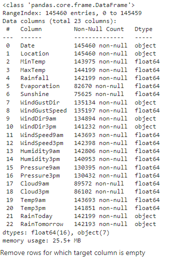
There are 145460 samples out of which there are 142193 samples whose 'RainTomorrow' column is non-null. Therefore, we can just remove the rows in which the 'RainTomorrow' column is null since there will be no significant information loss.

raw_df.dropna(subset=['RainTomorrow'], inplace=True)

6. Train, Validation, Test Split

Let us now learn what time-series data is !
Time series data is a collection of observations obtained through repeated measurements over time. Plot the points on a graph, and one of your axes would always be time.

The given data is a time-series data and is in chronological form. While working with chronological data, it's often a good idea to separate the training, validation and test sets with time, so that the model is trained on data from the past and evaluated on data from the future.

plt.title('No. of Rows Per Year');
sns.countplot(x=pd.to_datetime(raw_df.Date).dt.year);

We'll use the data till 2014 for the training set, data from 2015 for the validation set, and the data from 2016 & 2017 for the test set.

To do so,

year = pd.to_datetime(raw_df.Date).dt.year

train_df = raw_df[year < 2015]
val_df = raw_df[year == 2015]
test_df = raw_df[year > 2015]

7. Identify Inputs & Target Columns

The columns other than RainTomorrow are independent columns (input columns) while the RainTomorrow column is dependent column (output columns).

input_cols = list(train_df.columns[1:-1])
target_cols = train_df.columns[-1]

input_cols,target_cols

(['Location',
  'MinTemp',
  'MaxTemp',
  'Rainfall',
  'Evaporation',
  'Sunshine',
  'WindGustDir',
  'WindGustSpeed',
  'WindDir9am',
  'WindDir3pm',
  'WindSpeed9am',
  'WindSpeed3pm',
  'Humidity9am',
  'Humidity3pm',
  'Pressure9am',
  'Pressure3pm',
  'Cloud9am',
  'Cloud3pm',
  'Temp9am',
  'Temp3pm',
  'RainToday'],
 'RainTomorrow')

Identify inputs and outputs

• X_train : Training data's inputs

• Y_train : Training data's output
  Similarly for validation and test data.

X_train = train_df[input_cols].copy()
Y_train = train_df[target_cols].copy()

X_val = val_df[input_cols].copy()
Y_val = val_df[target_cols].copy()

X_test = test_df[input_cols].copy()
Y_test = test_df[target_cols].copy()

8. Identify Numerical & Categorical Columns

From the info of the dataset shown above, the Dtype column specifies the datatype of the column values. Different preprocessing steps are to be carried out for categorical data and numerical data. Hence we'll identify the columns which are numerical and which are categorical for preprocessing purposes.

numeric_cols = list(X_train.select_dtypes(include=np.number).columns)
categorical_cols = list(X_train.select_dtypes(include='object').columns)

numeric_cols, categorical_cols

(['MinTemp',
  'MaxTemp',
  'Rainfall',
  'Evaporation',
  'Sunshine',
  'WindGustSpeed',
  'WindSpeed9am',
  'WindSpeed3pm',
  'Humidity9am',
  'Humidity3pm',
  'Pressure9am',
  'Pressure3pm',
  'Cloud9am',
  'Cloud3pm',
  'Temp9am',
  'Temp3pm'],
 ['Location', 'WindGustDir', 'WindDir9am', 'WindDir3pm', 'RainToday'])

9. Impute Missing Values

As we have discussed already that preprocessing steps are to be done separately for numerical and categorical columns. First, let's impute the numerical columns with mean of the corresponding columns.

Below code displays the counts of null values in numerical columns sorted in descending order.

X_train[numeric_cols].isna().sum().sort_values(ascending=False)

Below code imputes the numerical columns with their mean respectively.

imputer = SimpleImputer(strategy='mean')
imputer.fit(raw_df[numeric_cols])

X_train[numeric_cols] = imputer.transform(X_train[numeric_cols])
X_val[numeric_cols] = imputer.transform(X_val[numeric_cols])
X_test[numeric_cols] = imputer.transform(X_test[numeric_cols])

Now, after imputing the null values with mean, the count of null values are :

X_train[numeric_cols].isna().sum().sort_values(ascending=False)

10. Scaling Numerical Columns

Let's learn the necessity of scaling before proceeding.
Feature Scaling is a technique to standardize the independent features present in the data in a fixed range. It is performed during the data pre-processing to handle highly varying magnitudes or values or units. If feature scaling is not done, then a machine learning algorithm tends to weigh greater values, higher and consider smaller values as the lower values, regardless of the unit of the values.

Example: If an algorithm is not using the feature scaling method then it can consider the value 3000 meters to be greater than 5 km but that’s actually not true and in this case, the algorithm will give wrong predictions. So, we use Feature Scaling to bring all values to the same magnitudes and thus, tackle this issue.

We'll use Min-Max Scaling to perform feature scaling.

To do so,

scaler = MinMaxScaler()
scaler.fit(raw_df[numeric_cols])

X_train[numeric_cols] = scaler.transform(X_train[numeric_cols])
X_val[numeric_cols] = scaler.transform(X_val[numeric_cols])
X_test[numeric_cols] = scaler.transform(X_test[numeric_cols])

11. Encoding Categorical Columns

Let's now learn what is encoding and why it is needed? Encoding categorical data is a process of converting categorical data into integer format so that the data with converted categorical values can be provided to the models to give and improve the predictions.

Every machine learning models learns only from numerical data which is why it is needed to convert the categorical data to integer format during preprocessing.

The categorical columns in our dataset are,

['Location', 'WindGustDir', 'WindDir9am', 'WindDir3pm', 'RainToday']

Note : Before encoding the categorical columns it is must to make sure that there are no null values in those columns because those columns will also be encoded which doesn't make sense. Therefore, the null values in categorical columns should be imputed before encoding the columns. This is similar to imputing numerical columns followed by scaling them.

Below code displays the count of null values in the categorical columns :

X_train[categorical_cols].isna().sum().sort_values(ascending=False)

It is also to be noted, imputing is done by considering mean in numerical columns. But this is not the case for categorical columns. For categorical columns either mode can be considered or some other dummy value can be substituted in place of null values. Here, let's substitue 'Unknown' in place of null values. To do so,

X_train[categorical_cols] = X_train[categorical_cols].fillna('Unknown')
X_val[categorical_cols] = X_val[categorical_cols].fillna('Unknown')
X_test[categorical_cols] = X_val[categorical_cols].fillna('Unknown')

Now the counts of null values are :

X_train[categorical_cols].isna().sum().sort_values(ascending=False)

Coming back, after imputing the null values let's perform encoding.

encoder = OneHotEncoder(sparse=False, handle_unknown='ignore')
encoder.fit(X_train[categorical_cols])

encoded_cols = list(encoder.get_feature_names(categorical_cols))
encoded_cols

['Location_Adelaide',
 'Location_Albany',
 'Location_Albury',
 'Location_AliceSprings',
 'Location_BadgerysCreek',
 'Location_Ballarat',
 'Location_Bendigo',
 'Location_Brisbane',
 'Location_Cairns',
 'Location_Canberra',
 'Location_Cobar',
 'Location_CoffsHarbour',
 'Location_Dartmoor',
 'Location_Darwin',
 'Location_GoldCoast',
 'Location_Hobart',
 'Location_Katherine',
 'Location_Launceston',
 'Location_Melbourne',
 'Location_MelbourneAirport',
 'Location_Mildura',
 'Location_Moree',
 'Location_MountGambier',
 'Location_MountGinini',
 'Location_Newcastle',
 'Location_Nhil',
 'Location_NorahHead',
 'Location_NorfolkIsland',
 'Location_Nuriootpa',
 'Location_PearceRAAF',
 'Location_Penrith',
 'Location_Perth',
 'Location_PerthAirport',
 'Location_Portland',
 'Location_Richmond',
 'Location_Sale',
 'Location_SalmonGums',
 'Location_Sydney',
 'Location_SydneyAirport',
 'Location_Townsville',
 'Location_Tuggeranong',
 'Location_Uluru',
 'Location_WaggaWagga',
 'Location_Walpole',
 'Location_Watsonia',
 'Location_Williamtown',
 'Location_Witchcliffe',
 'Location_Wollongong',
 'Location_Woomera',
 'WindGustDir_E',
 'WindGustDir_ENE',
 'WindGustDir_ESE',
 'WindGustDir_N',
 'WindGustDir_NE',
 'WindGustDir_NNE',
 'WindGustDir_NNW',
 'WindGustDir_NW',
 'WindGustDir_S',
 'WindGustDir_SE',
 'WindGustDir_SSE',
 'WindGustDir_SSW',
 'WindGustDir_SW',
 'WindGustDir_Unknown',
 'WindGustDir_W',
 'WindGustDir_WNW',
 'WindGustDir_WSW',
 'WindDir9am_E',
 'WindDir9am_ENE',
 'WindDir9am_ESE',
 'WindDir9am_N',
 'WindDir9am_NE',
 'WindDir9am_NNE',
 'WindDir9am_NNW',
 'WindDir9am_NW',
 'WindDir9am_S',
 'WindDir9am_SE',
 'WindDir9am_SSE',
 'WindDir9am_SSW',
 'WindDir9am_SW',
 'WindDir9am_Unknown',
 'WindDir9am_W',
 'WindDir9am_WNW',
 'WindDir9am_WSW',
 'WindDir3pm_E',
 'WindDir3pm_ENE',
 'WindDir3pm_ESE',
 'WindDir3pm_N',
 'WindDir3pm_NE',
 'WindDir3pm_NNE',
 'WindDir3pm_NNW',
 'WindDir3pm_NW',
 'WindDir3pm_S',
 'WindDir3pm_SE',
 'WindDir3pm_SSE',
 'WindDir3pm_SSW',
 'WindDir3pm_SW',
 'WindDir3pm_Unknown',
 'WindDir3pm_W',
 'WindDir3pm_WNW',
 'WindDir3pm_WSW',
 'RainToday_No',
 'RainToday_Unknown',
 'RainToday_Yes']

X_train[encoded_cols] = encoder.transform(X_train[categorical_cols])
X_val[encoded_cols] = encoder.transform(X_val[categorical_cols])
X_test[encoded_cols] = encoder.transform(X_test[categorical_cols])

Now, let's combine the preprocessed numerical and categorical columns for model training !!!

X_train = X_train[numeric_cols + encoded_cols]
X_val = X_val[numeric_cols + encoded_cols]
X_test = X_test[numeric_cols + encoded_cols]

12. Training & Visualizing Decision Trees

A decision tree in machine learning works in exactly the same way, and except that we let the computer figure out the optimal structure & hierarchy of decisions, instead of coming up with criteria manually.

Being a classification task, let's use DecisionTreeClassifier algorithm !!!

Training

model = DecisionTreeClassifier(random_state = 42)
model.fit(X_train, Y_train)

Now, we have trained our classifier with the training data.

Evaluation

To evaluate the training process, let's check how well the model trained with the training data.

X_train_pred = model.predict(X_train)
pd.value_counts(X_train_pred)

The counts of predicted result shows that our model has predicted more 'No' for the target column RainTomorrow than that of 'Yes'.

Now, let's calculate the accuracy of our model in the training data itself.

train_probs = model.predict_proba(X_train)
print('Training Accuracy :',accuracy_score(X_train_pred,Y_train)*100)

Training Accuracy : 99.99797955307714

Whooooaa !!! The training set accuracy is close to 100%! But we can't rely solely on the training set accuracy, we must evaluate the model on the validation set too. This is because our model should be trained in a generalized way i.e, it should be able to predict output which is not present in training data.

print('Validation Acuracy :',model.score(X_val,Y_val)*100)

Validation Acuracy : 79.28152747954267

Let's also calculate the percentage of 'Yes' and 'No' in validation data.

Y_val.value_counts() / len(Y_val)

The above result shows that, there are 78.8% 'No' and 21% 'Yes' in validation data. This proves that, if it is predicted 'No' for all the validation data, it would still be 78.8% accurate in the result (since there are 78.8% 'No' in the validation data). Therefore, our model should be considered learning only if it exceeds 78.8% accuracy because even predicting 'No' always using a dumb model gives 78.8% accuracy.

Conclusion :

• The training accuracy is 100%

• The validation accuracy is 79%

• Percentage of No in validation data is 78.8%

• Therefore, our model is only marginally better then always predicting "No"

The reason for this is that the training data from which our model learnt is skewed towards 'No'.

Note : Decision trees overfits !!!

Visualization of Decision Tree

plt.figure(figsize=(80,50))
plot_tree(model, feature_names=X_train.columns, max_depth=2, filled=True);

13. Feature Importance

The initial 23 columns (or features) after encoding became 119 features. Decision Trees can find importance of features by itself. Below are some of the importances of 119 features(total number of features in the training dataset).

feature_importance_df = pd.DataFrame({
    'Feature' : X_train.columns,
    'Importance' : model.feature_importances_
}).sort_values(by='Importance', ascending=False)
feature_importance_df

Note : Only some feature importances are displayed but the above code displays for all features.

Let's view importances of top 20 features.

plt.title('Feature Importance')
sns.barplot(data = feature_importance_df.head(20), x='Importance', y='Feature');

14. Hyperparameter Tuning - To Reduce Overfitting

Since we have found out that our model is only marginally better than a dumb model because of overfitting, we should modify some of the parameters of DecisionTreeClassifier to reduce overfitting.

The DecisionTreeClassifier accepts several arguments, some of which can be modified to reduce overfitting.

• max_depth

• max_leaf_nodes

By reducing the tree maximum depth can reduce overfitting. Maximum depth (default) is 48 which is reduced to 3 to reduce overfittting as below.

model = DecisionTreeClassifier(random_state=42, max_depth=3)
model.fit(X_train, Y_train)

print('Accuracy in Training Dataset :',model.score(X_train, Y_train)*100)
print('Accuracy in Validation Dataset :',model.score(X_val, Y_val)*100)

Accuracy in Training Dataset : 82.91308037337859
Accuracy in Validation Dataset : 83.34397307178921

Tuning max_depth

Since the max_depth value without manual constraint for which our model overfitted is 48. And the max_depth value obviously can't be 0 (or lesser). So let's find what the best value of max_depth would be by trial and error method and use the max_depth for which the errors of train and validation dataset is optimal.

def max_depth_accuracy1(max_depth_val):
    model = DecisionTreeClassifier(random_state=42, max_depth=max_depth_val)
    model.fit(X_train, Y_train)
    train_accuracy = model.score(X_train, Y_train)*100
    val_accuracy = model.score(X_val, Y_val)*100
    return {'Max_Depth' : max_depth_val, 'Training_Accuracy' : train_accuracy, 'Validation_Accuracy' : val_accuracy}

accuracies_df1 = pd.DataFrame([max_depth_accuracy1(i) for i in range(1,48)])
accuracies_df1

From the dataframe, it can be seen that the training accuracy increases with increase in max_depth. It is also to be noted that validation accuracy first increases and then decreases.

Tuning Graph

Let'us visualise the training accuracy and validation accuracy with different max_depths.

plt.title('Training Accuracy Vs Validation Accuracy');
plt.plot(accuracies_df1['Max_Depth'], accuracies_df1['Training_Accuracy']);
plt.plot(accuracies_df1['Max_Depth'], accuracies_df1['Validation_Accuracy']);
plt.legend(['Training Accuracy', 'Validation Accuracy']);
plt.xticks(range(0,48, 2))
plt.xlabel('Max Depth');
plt.ylabel('Errors');

From the graph it can also be seen that training accuracy increases with increase in max_depth while validation accuracy first increases (till max_depth = 7) and then decreases. Therefore, optimal max_depth is 7.

Build Decision Tree with max_depth = 7

model = DecisionTreeClassifier(random_state=42, max_depth=7)
model.fit(X_train, Y_train)
print('Training Accuracy :', model.score(X_train,Y_train)*100)
print('Validation Accuracy :', model.score(X_val, Y_val)*100)

Training Accuracy : 84.66884874934335
Validation Accuracy : 84.53949277465034

Tuning max_leaf_nodes

Another way to control the size of complexity of a decision tree is to limit the number of leaf nodes. This allows branches of the tree to have varying depths. Let's limit the number of leaf nodes to 128 at maximum.

model = DecisionTreeClassifier(max_leaf_nodes=128, random_state=42)
model.fit(X_train, Y_train)
print('Training Accuracy :', model.score(X_train,Y_train)*100)
print('Validation Accuracy :', model.score(X_val, Y_val)*100)

Training Accuracy : 84.80421869317493
Validation Accuracy : 84.42342290058616

Let's see the accuracies when max_leaf_nodes was set to 128 (at maximum).

accuracies_df1.loc[accuracies_df1['Max_Depth'] == model.tree_.max_depth]

Now, let's train our DecisionTreeClassifier with max_leaf_nodes = 128 and max_depth = 6,

model = DecisionTreeClassifier(max_leaf_nodes=128, random_state=42, max_depth=6)

Let's now use the trial and error method considering the two parameters,

def max_depth_accuracy2(max_depth_val):
    model = DecisionTreeClassifier(random_state=42, max_depth=max_depth_val, max_leaf_nodes=128)
    model.fit(X_train, Y_train)
    train_accuracy = model.score(X_train, Y_train)*100
    val_accuracy = model.score(X_val, Y_val)*100
    return {'Max_Depth' : max_depth_val, 'Training_Accuracy' : train_accuracy, 'Validation_Accuracy' : val_accuracy}

accuracies_df2 = pd.DataFrame([max_depth_accuracy2(i) for i in range(1,14)])
accuracies_df2

Tuning Graph

Let'us visualise the training accuracy and validation accuracy with different max_depths and max_leaf_nodes = 128.

plt.title('Training Accuracy Vs Validation Accuracy');
plt.plot(accuracies_df2['Max_Depth'], accuracies_df2['Training_Accuracy']);
plt.plot(accuracies_df2['Max_Depth'], accuracies_df2['Validation_Accuracy']);
plt.legend(['Training Accuracy', 'Validation Accuracy']);
plt.xticks(range(0,16, 2))
plt.xlabel('Max Depth');
plt.ylabel('Errors');

It seems max_depth = 9 and max_leaf_nodes = 128 is the optimal hyperparameters

Now, let's train our classifier with the best found hyperparameters,

model = DecisionTreeClassifier(max_depth=9, max_leaf_nodes=128, random_state=42)
model.fit(X_train, Y_train)
print('Training Accuracy :', model.score(X_train,Y_train)*100)
print('Validation Accuracy :', model.score(X_val, Y_val)*100)

Training Accuracy : 84.89614902816504
Validation Accuracy : 84.46404735650862

You can find the code on my Github : avinash-218

---

Connect me through :

• LinkedIn

• GitHub

• Instagram

Feel free to correct me !! :)
Thank you folks for reading. Happy Learning !!! 😊