Index
1. Problem Statement
2. Dataset Description
3. Artificial Neural Network Implementation
3.1. Import Libraries & Dependencies
3.2. Import Dataset
3.3. Data Preprocess
3.4. Normalize the Data
3.5. Train Test Split
3.6. Model Training
3.7. Model Evaluation
3.8. Testing
3.9. Save Model & Weights
4. Artificial Neural Network Implementation with Feature extraction
5. Convolutional Neural Network Implementation
6. Results Comparisons
7. Author
1. Problem Statement
In this article, we will be using Artificial Neural Network (ANN), Convolutional Neural Networks (CNN) and ANN with Feature Extraction to perform binary classification of Homer and Bart Images to compare the result and time taken by each method to practically prove why CNN is preferred for image data.
2. Dataset Description
We'll use the image dataset of Homer and Bart in this article. The dataset can be taken from Kaggle. The Simpsons - Bart and Homer Data The dataset consists of Homer and Bart images.
3. Artificial Neural Network Implementation
The implementation code is available in my GitHub account. Repository Link: Homer Vs Bart ANN. We'll go through step by step explanation of the code.
3.1 Import Libraries & Dependencies
Initially, let's import the necessary libraries.
import os
import cv2
import seaborn as sns
import numpy as np
from sklearn.preprocessing import MinMaxScaler
from sklearn.model_selection import train_test_split
from sklearn.metrics import accuracy_score, confusion_matrix, classification_report
import tensorflow as tf
import pandas as pd
import matplotlib.pyplot as plt
from keras.models import save_model
3.2 Import Dataset
directory = '../input/homerbart1/homer_bart_1'  #path of extracted dataset (current location)
files = [os.path.join(directory, f) for f in sorted(os.listdir(directory))] #contains paths of each images
directory variable specifies the path of the dataset images folder;
files variable contains the file names of the images;
3.3 Data Preprocessing
height, width = 128, 128   #since all images are of different shapes reshape them to this shape
images =[]  #pixel values of all images
classes = []    #class of all images
Each images are of a different size, so we'll reshape them to equal size - (128, 128). images variable consists of image pixel values;
classes variable denotes the class of each image;
for image_path in files:
    try:    #exception handling for the irrelevant file DSstore that is in the directory (shortly can delete the file)
        image = cv2.imread(image_path)  #read image one by one
        (H, W) = image.shape[:2]    #since this is RGB image need only first two values are height and weight
    except:
        continue

    image = cv2.resize(image, (width, height))  #resize the image to 128,128,3
    image = cv2.cvtColor(image, cv2.COLOR_BGR2GRAY) #convert to gray scale
    image = image.ravel()       #convert matrix to vector to feed to input layer
    images.append(image)    #store all vector representation of images

    image_name = os.path.basename(os.path.normpath(image_path)) #extract only filename

    if(image_name.startswith('b')): #encoding categorical data
        class_name = 0  #bart - 0
    else:
        class_name = 1  #homer -1

    classes.append(class_name)  #store all class_names
The above code snippet reads images from the path and performs preprocessing like resizing, converting to gray scale, flatten the array. ravel() is used to flatten the image from 2D array to 1D array. After such preprocessing, the pixel values are appended to the list denoted by the variable image.
Also, labels of each file are extracted based on file names. The images starting with the file name ' b' (denoting 'Bart' images) are labeled as class 0 while the images starting with file name 'h' (denoting 'Homer' images) are labeled as class 1. The classes are appended to the variable classes.
Now, we'll convert images and classes variables to numpy representation for further processing compatibility and for ease of use.
X = np.asarray(images)  #or can use X = np.array(images)
Y = np.asarray(classes) #or can use Y = np.array(classes)
3.4 Normalize the data
scaler = MinMaxScaler()
X = scaler.fit_transform(X)                 #or just divide X by 255
Pixel values are then scaled using a min-max scaler for normalization.
3.5 Train Test Split
Let's split the entire data into training data (80%) and testing data (20%). The model is trained using the training data and the trained model is evaluated using testing data.
X_train, X_test, Y_train, Y_test = train_test_split(X, Y, test_size=0.2, random_state = 1) #20% data as test data
3.6 Train Model
Now comes the model training, blindly let's specify the number of neurons in the hidden layer as the average of input and output layer units. The input layer gets images of 128x128 values each as a single dimension vector (since we have flattened the 2d array using the ravel() method). Therefore, there are 16384 neurons in the input layer. Also, since we are dealing with binary classification, the output layer consists of 1 neuron.
Model Configurations:
Input Layer Units: 16384
Output Layer Units: 1
Number of Hidden Layers: 3
Activation Function (Hidden Layers):
reluActivation Function (Output Layer):
sigmoidOptimizer:
AdamLoss:
Binary Cross-EntropyMetric:
AccuracyEpochs: 50
network1 = tf.keras.models.Sequential()
network1.add(tf.keras.layers.Dense(input_shape=(X_train.shape), units = 8193, activation='relu'))
network1.add(tf.keras.layers.Dense(units = 8193, activation='relu'))    #2nd layer
network1.add(tf.keras.layers.Dense(units=1, activation='sigmoid'))  #since binary classification sigmoid activation
Then comes model compilation,
network1.compile(optimizer='Adam', loss='binary_crossentropy', metrics=['accuracy'])
Training for 50 epochs...
history = network1.fit(X_train, Y_train, epochs = 50)
3.7 Model Evaluation
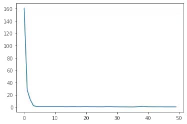
Let's visualize the loss degradation concerning epochs.
print(history.history.keys())
plt.plot(history.history['loss']);
3.8 Testing
Let's test our model performance with the test data set.
predictions = network1.predict(X_test)

#convert predictions (probabilities) to classes
predictions = (predictions > 0.5) #threshold = 0.5

#test evaluation
print('Accuracy :', accuracy_score(predictions, Y_test)*100)
cm = confusion_matrix(Y_test, predictions)
Accuracy: 53.70370370370371
Confusion Matrix,
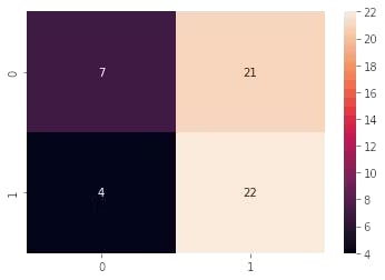
The classification report of the model on the test data is,
print(classification_report(Y_test, predictions))

         precision    recall  f1-score   support

           0       0.64      0.25      0.36        28
           1       0.51      0.85      0.64        26

    accuracy                           0.54        54
   macro avg       0.57      0.55      0.50        54
weighted avg       0.58      0.54      0.49        54
3.9 Save Model & Weights
Let's save the model in .json format and the trained weights in .hdf5 format.
#save json model structure
model_json = network1.to_json()   #convert model to json format
with open('network1.json', 'w') as json_file:
  json_file.write(model_json) #write the json format of model to network1.json file

#save model weights
network1_saved = tf.keras.models.save_model(network1, 'weights1.hdf5')
This is the end of Artificial Neural Networks for binary image classification. The results will be revisited in the upcoming sections for comparison purposes.
4. Artificial Neural Network Implementation with Feature extraction
Let's move directly to the core concept of feature extraction since the overall flow is covered in the previous section. Refer to the GitHub code for full code - ANN + Feature Extraction
The feature extraction considered is based on the colors. Let's take some sample images of Homer and Bart to distinguish them only based on colors. Note: The features are extracted only based on colors and not based on any other factors like shape, size etc...

The following code snippet performs the feature extraction of the classes based on colors. Z in (X, Y, Z) is the channel of the image. Since we are dealing with BGR,
Z=0=> Blue;
Z=1=>Green;
Z=2=> Red.
Therefore, we extract each channel's intensity and compare them with a set of pre-determined colors which are helpful to distinguish Homer and Bart. Here, we have considered the colors of the mouth, pants, and shoes of Homer as the features and colored them yellow to visualize the result. Similarly, we have considered the colors of t-shirts, shorts, and sneakers of Bart as features and colored them with green color to visualize the result.
#go through each pixel one by one to extract colors of each pixel
  for height in range(0,H): #each pixel in height
    for width in range(0, W): #each pixel in width
      blue = image.item(height, width, 0)     #extract value from height,width (location) and 0th channel in BGR which is blue channel
      green = image.item(height, width, 1)     #extract value from height,width (location) and 1st channel in BGR which is green channel
      red = image.item(height, width, 2)     #extract value from height,width (location) and 2nd channel in BGR which is red channel

      #Homer - brown(mouth)
      if(blue>=95 and blue<=140 and green >=160 and green <=185 and red >= 175 and red <= 200):
        image[height,width] = [0,255,255]   #color the pixel with yellow color
        mouth+=1  #incrementing that one pixel has the color of the feature

      #Homer - blue (pants)
      if(blue>=150 and blue<=180 and green >=98 and green <=120 and red >= 0 and red <= 90):
        image[height,width] = [0,255,255]   #color the pixel with yellow color
        pants+=1

      #Homer - gray(shoes)
      if(height > (H/2)):   #since shoes are present only at bottom only considering lower part of image
        if(blue>=25 and blue<=45 and green >=25 and green <=45 and red >= 25 and red <= 45):
          image[height,width] = [0,255,255]   #color the pixel with yellow color
          shoes+=1

      #Bart - orange (tshirt)
      if(blue>=11 and blue<=22 and green >=85 and green <=105 and red >= 240 and red <= 255):
        image[height,width] = [0,255,0]   #color the pixel with green color
        tshirt+=1

      #Bart - blue (shorts)
      if(blue>=125 and blue<=170 and green >=0 and green <=12 and red >= 0 and red <= 20):
        image[height,width] = [0,255,0]   #color the pixel with green color
        shorts+=1

      #Bart - blue (sneakers)
      if(height > (H/2)):   #since sneakers are present only at bottom only considering lower part of image
        if(blue>=125 and blue<=170 and green >=0 and green <=12 and red >= 0 and red <= 20):
          image[height,width] = [0,255,0]   #color the pixel with green color
          sneakers+=1
The below code snippet normalizes the feature area with a total number of pixels. Eg: Consider we have 100x200 pixels of an image (20000 pixels) and 2000 of the pixels are detected to have a mouth feature so (2000 / 20000) x 100 = 10 i.e,10% of the image we have pixels to detect the mouth feature
  mouth = round((mouth / (H*W))*100,9)
  pants = round((pants / (H*W))*100,9)
  shoes = round((shoes / (H*W))*100,9)
  tshirt = round((tshirt / (H*W))*100,9)
  shorts = round((shorts / (H*W))*100,9)
  sneakers = round((sneakers / (H*W))*100,9)

#appending features in a image to image_features
  image_features.append(mouth)
  image_features.append(pants)
  image_features.append(shoes)
  image_features.append(tshirt)
  image_features.append(shorts)
  image_features.append(sneakers)

#appending class names to image_features
  image_features.append(class_name)

#appending image_features to features (which contains all features of all images)
  features.append(image_features)
Now, after extracting the features, let's store them as a comma-separated value format.
with open('features.csv', 'w') as file:
  for l in export:
    file.write(l)
file.closed
After saving the extracted features as a CSV file, let's build our ANN model to classify the images.
Loading data and extracting input (X) and label (Y) and train-test-split is given below,
dataset = pd.read_csv('../input/featuresbart-homer/features.csv')
#Extract X and Y
X = dataset.iloc[:,:-1].values
Y = dataset.iloc[:,-1].values

X_train, X_test, Y_train, Y_test = train_test_split(X, Y, test_size = 0.2, random_state = 1)
Now comes the model building, Since we have only considered 6 features (i.e., mouth, pants, shoes of Homer and t-shirt, shorts, sneakers of Bart), the input layer only required 6 neurons. Similar model configurations are used here as well.
network1 = tf.keras.models.Sequential()
network1.add(tf.keras.layers.Dense(input_shape = (6,), units = 4, activation='relu'))
network1.add(tf.keras.layers.Dense(units = 4, activation='relu'))
network1.add(tf.keras.layers.Dense(units = 4, activation='relu'))
network1.add(tf.keras.layers.Dense(units = 1, activation='sigmoid'))
The results of the training are as follows,
Accuracy: 87.03703703703704
Classification Report:
 precision    recall  f1-score   support

           0       0.96      0.79      0.86        28
           1       0.81      0.96      0.88        26

    accuracy                           0.87        54
   macro avg       0.88      0.87      0.87        54
weighted avg       0.88      0.87      0.87        54
Confusion Matrix:
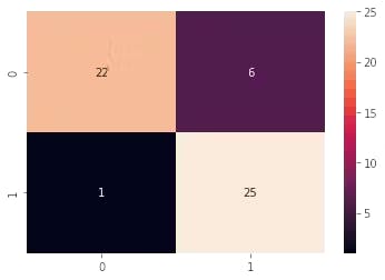
This is the end of Artificial Neural Network + Feature Extraction for binary image classification. We can see that accuracy has risen!!!.... Let's now dive into Convolutional Neural Networks to see how will be the results.
5. Convolutional Neural Network Implementation
Only core concepts are discussed here to avoid redundancy. Check out this GitHub link for the entire code: Homer Vs Bart - CNN
Let's use the ImageDataGenerator to load our images. The augmentation implemented are scaling, rotation, horizontal flips and zooming.
train_generator = ImageDataGenerator(rescale = 1./255,  #generate train images
                                     rotation_range=7,
                                     horizontal_flip=True,
                                     zoom_range=0.2)

train_dataset = train_generator.flow_from_directory('../input/homerbart2/homer_bart_2/training_set',
                                                    target_size=(64, 64),
                                                    batch_size = 8,
                                                    class_mode='categorical',
                                                    shuffle=True)
test_generator = ImageDataGenerator(rescale = 1./255)

test_dataset = test_generator.flow_from_directory('../input/homerbart2/homer_bart_2/test_set',
                                                  target_size=(64,64),
                                                  batch_size=1,
                                                  class_mode='categorical',
                                                  shuffle=False)
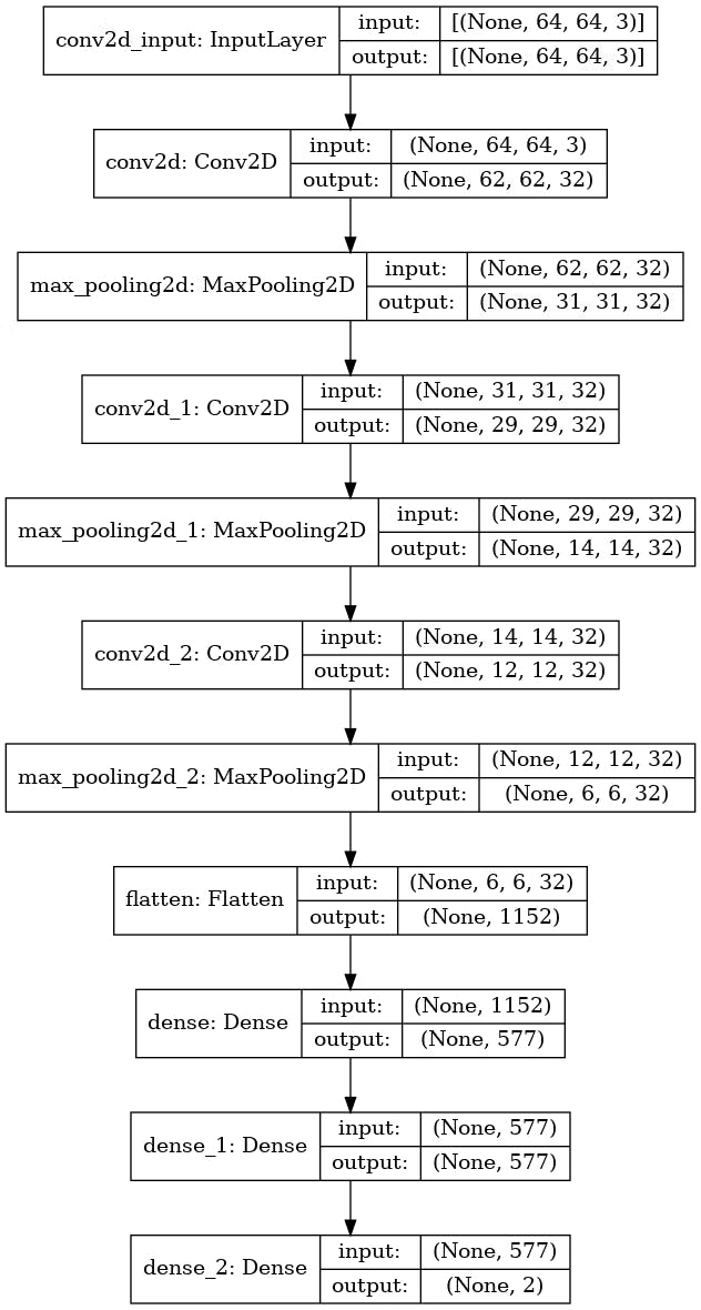
Let's now build our CNN model for the same classification task,
model = Sequential()

model.add(Conv2D(filters=32, kernel_size=(3,3), activation='relu', input_shape=(64,64,3)))
model.add(MaxPooling2D(2,2))

model.add(Conv2D(filters=32, kernel_size=(3,3), activation='relu'))
model.add(MaxPooling2D(2,2))

model.add(Conv2D(filters=32, kernel_size=(3,3), activation='relu'))
model.add(MaxPooling2D(2,2))

model.add(Flatten())    #1152 outputs
#(1152 + 2)/2 = 577
model.add(Dense(units=577, activation='relu'))
model.add(Dense(units=577, activation='relu'))
model.add(Dense(units=2, activation='softmax'))
Model Summary,
model.summary()
tf.keras.utils.plot_model(model, to_file='Model.png', show_shapes=True)
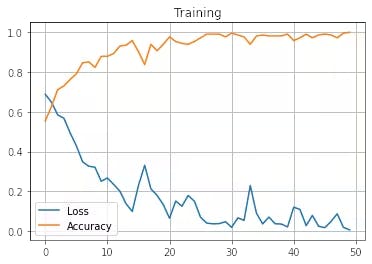
Visualizing the training results,
plt.plot(model_history.history['loss'])
plt.plot(model_history.history['accuracy'])
plt.grid(True)
plt.legend(['Loss','Accuracy'])
plt.title('Training')
plt.savefig('Training.jpg')
Evaluation of the test data set.
predictions = model.predict(test_dataset)

#since we used categorical model(not binary) we get probabilities for an image to be in each class
#so we consider that the image belogs to the class with higher probability
#print(predictions)
predictions = np.argmax(predictions, axis=1)

#print(test_dataset.classes) #expected classes
#print('\n',predictions) #predicted classes

print('Accuracy :',accuracy_score(predictions,test_dataset.classes)*100)    #accuracy
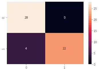
cm = confusion_matrix(test_dataset.classes, predictions)
sns.heatmap(cm, annot=True)
print(classification_report(test_dataset.classes, predictions))
Accuracy: 92.5925925925926
Classification Report:
 precision    recall  f1-score   support

           0       0.88      1.00      0.93        28
           1       1.00      0.85      0.92        26

    accuracy                           0.93        54
   macro avg       0.94      0.92      0.93        54
weighted avg       0.94      0.93      0.93        54
Confusion Matrix
This is the end of the Convolutional Neural Network for binary image classification. We can see that accuracy has risen a lot!!!.... Let's now compare the results and come to a conclusion.
6. Results Comparison
To summarize, this blog considered the Homer - Bart image dataset for the classification task. The dataset is classified by using Artificial Neural Networks, Artificial Neural Networks with Feature Extraction and Convolutional Neural Networks. We have seen (so far) that accuracy has risen. This section compares factors other than accuracy scores for image classification and concludes.
Implementation / Factors | Training Time | Weight Storage | Accuracy |
ANN | Very High | Around 25 GB | 53.70370370370371 |
ANN+Feature Extraction | Lesser than ANN | Few KBs | 87.03703703703704 |
CNN | Very Less | Few KBs | 92.5925925925926 |
From the table above, it can be seen that in terms of Training Time, Space occupied by trained weights and accuracy, Convolutional Neural Networks have the bigger hand. Therefore, this proves why CNNs are considered to be the best while dealing with image datasets.
7. Author
You can find the code on my Github: Homer-Bart-Classification-ANN-Feature-Extraction-CNN-Transfer-Learning
About the Author :
Hiii, I'm Avinash, pursuing a Bachelor of Engineering in Computer Science and Engineering from Mepco Schlenk Engineering College, Sivakasi. I'm an AI enthusiast and Open-Source contributor.
Connect me through :
Feel free to correct me !! :)
Thank you folks for reading. Happy Learning !!! 😊
